1) Double-click on the simulation icon to start the exercise.
2) After a few seconds, a window will appear. This includes a satellite image, as well as several variables describing fishery biology and economics, and simulation General parameters (see Glossary).
3) There are three species-types to choose from. These are grouper, conch, and lobster. Their characteristics are based on those of real organisms.
4) Each variable (for example: lifespan) is set to default values that are within ranges published in the literature for the focal species, when these are known (Table 1). It is important to note that the exercise simulates "species types" and their fisheries. As such, the simulated organisms and their fisheries, although generally similar to grouper, conch, and spiny lobsters, are not intended to represent real world situations. To simulate other organisms of your choice, you can alter these numbers by selecting them and typing in your own values.
| Grouper | Conch | Lobster | |
| Initial population | 50,000 | 150,000 | 110,000 |
| Lifespan (days) | 3285 | 3102 | 2920 |
| Intrinsic growth rate | 0.2 | 0.4 | 0.5 |
| Carrying capacity | 10000 | 15000 | 12500 |
| Avg. catch weight (kg) | 5 | 0.4 | 1 |
| Dispersal rate | 8 | 1 | 6 |
| Fishing efficiency | 0.02 | 0.09 | 0.04 |
| Speed (km/hr) | 20 | 20 | 20 |
| Travel cost ($/km ) | 1 | 1 | 1 |
| Boat cost ($/day ) | 12 | 12 | 12 |
| Max. boats/port | 35 | 35 | 35 |
| Maximum harvest (kg) | 200 | 40 | 100 |
| Price ($/kg) | 5 | 6 | 8 |
Table 1. Summary of default values employed in the simulation exercise.
5) Pointing at each parameter with your cursor causes tool tips to appear. These explain each parameter, and provide minimum and maximum values. Parameters are also described in the Glossary. Please note: these tool tips will only appear if your mouse is rolled over the value legend (such as "Initial population" or "Lifespan (days)". The tool tips will not appear if the mouse is rolled over the value field, or boxes where the variables are set.
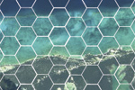
6) You will see that the base image is overlaid by a hexagonal grid. In conservation planning, landscapes or seascapes are often subdivided into such units for planning purposes.
7) The red dots in each hexagon reflect the relative abundance of adult organisms within each planning unit. Pointing at a planning unit with your cursor will cause the number of organisms present in the hexagon, as well as the habitat type (see below), to appear.
8) Later on in the exercise, you will be able to construct a reserve system by clicking on hexagonal planning units of your choice. This will cause the hexagon to become outlined in white. No fishing will occur in protected hexagons, although boats may transit through without fishing.
9) You will also be able to follow boat movements along the seascape. Boats belong to one of two ports (Yellow or Blue), and are represented by small dots of the corresponding colors.
10) Pressing the Run button will start the simulation.
11) You may interrupt the run by pressing the Stop button. The speed of the simulation can also be changed in the appropriate field. Please note that 100 is the maximum available speed (as noted in the tool tips). There are additional buttons to speed up the simulation by the chosen time period (for example, "+1 decade").
12) While the simulation is running, the base image will depict changes in numbers of adults through corresponding alterations in size of the red dots.
13) Changes in population numbers (total and within reserves), as well as economic aspects of the fishery are shown in 4 graphs. Please note that the scale of the graphs changes as the data warrant. Clicking on a graph will cause a larger version to appear in a separate window. The graphs can also be saved using the "Save" option in the "File" menu.
14) Boats exit the simulation if their profits are negative, so that boat numbers may vary throughout the run. This simulation assumes there will be at least one boat from each port participating in the fishery, even at negative profits. The model for the behavior of fishermen is that if all boats from a given port have negative profit one day, then one boat drops out of service. One or more boats can be making a profit, even while the average profit (shown in the graphs) is negative. Thus, the average profit can go negative for a while, before boats start dropping out of service, and more than one boat may be present even at negative profits.
15) The percentage of total area in reserves at any given time is shown on the bottom right of the panel, as are the number of days simulated. Both are highlighted in red.
16) The simulation will end automatically when either the maximum days simulated or the minimum population size are reached. The default value for maximum days simulated is 20 years (7300 days). These variables can be specified in the column headed "General Parameters" on the right hand side of the panel.
17) You may alter the base image of the simulation using the "Base image of display" button on the bottom right. Toggle between a satellite image, an image showing habitat classifications, and an image reflecting habitat suitability for each species type. Species occurrence in each kind of habitat is based on their biology. Sea grass is appropriate habitat for conch, for example, while coral reefs are more suitable for spiny lobsters and groupers. Pointing your cursor at any hexagon will cause these classifications to appear. In the suitability screen, the most suitable habitats are lighter in color. The habitats, classified as follows, are defined in the Glossary:
- Unclassified (land or deep water)
- Sparse seagrass
- Medium density seagrass
- Dense seagrass
- Sand
- Silt / mud
- Batophora dominated
- Sargassum on hardbottom
- Dead coral and Microdictyon
- Sparse gorgonians and algae
- Uncolonized pavement and sparse gorgonians
- Montastraea reef
- Acropora palmata reef
- Porites reef
- Patch reef
- Mangrove
18) The "Base image of display" menu also contains options that summarize the following simulation outputs: Average effort, Average harvest, Potential yellow or blue boat profits, and Yellow or Blue boat profit sources. Values corresponding to each cell are provided in the tool tips. The Average effort and Average harvest options output the average effort and catch over the last year of the simulation. The Potential profit displays reveal the projected profits for each color boat at the time. The profit source feature tracks the cells of origin (i.e., birth) for individuals that are caught by blue or yellow boats in fishable areas. The lighter colors indicate larger amounts, and the values corresponding to each cell are provided in the tool tips.
19) You can save your results by opening the File menu under the Save option, on the upper right hand side of the screen.
20) You will be able to Reset to Time 0, Clear reserves, or Reset default values by selecting these options under the Edit menu, on the upper left side of the screen.
21) If you would like to learn more about the simulation model, click here. The model can also be found in Appendix I at the end of the Exercise.
Although efforts have been made to provide a realistic scenario, due to necessary simplifications and model assumptions, simulation results are not intended to reflect reality.

